catalytic_reaction

Overview

This model defines the following ‘catalytic reaction’ system:

Here, the species acts as a catalyst for the third reaction. The rate constants are , and , while the initial species counts are , and .

This catalytic reaction system is taken from the paper by Mastny, Haseltine, Rawlings [MHR07] .

Running the model

This model is defined by the module cmepy.model.catalytic_reaction. The source code for this model is listed below.

The model solves the distribution over a sparse, truncated state space. For more information, see Sparse state spaces.

To run this model, open the Python interpreter, and enter:

>>> from cmepy.models import catalytic_reaction
>>> catalytic_reaction.main()

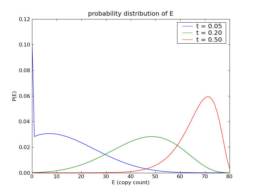
This will solve the model and then produce the following plot, illustrating the marginal distribution of species count of at the times .

Sample results

Source

"""
A simple catalytic reaction example.

Consider the following 'catalytic' reaction system:

    A --k_1--> B
    B --k_2--> C
    B + D --k_3--> B + E

Here, the species B acts as a catalyst for the third
reaction. The rate constants are

    k_1 = 1, k_2 = 1000, k_3 = 100;

while the initial species counts are

    A = 50, D = 80, B = C = E = 0.

This system is taken from the paper 

    Mastny, E.A., Haseltine, E.L. and Rawlings, J.B.
    Two classes of quasi-steady-state model reductions for stochastic kinetics,
    The Journal of Chemical Physics, 2007, Vol 127 .

"""

import numpy
import pylab

import cmepy.domain
import cmepy.model
import cmepy.solver
import cmepy.recorder
from cmepy.util import non_neg, consecutive_pairs

def gen_states(**initial_counts):
    """
    gen_states(**initial_counts) -> first state, ..., last state
    
    Creates a generator over states in a *truncated* reaction count state
    space, for the catalytic reaction example.
    
    If specified, the optional keyword arguments A (defaults to  50) and
    D (defaults to 80) define the initial copy counts of species A and D
    respectively.
    
    Each state yielded by this generator has the form state = (r_1, r_2, r_3),
    where non-negative integers r_1, r_2 and r_3 denote the count of the
    reactions 1, 2 and 3, respectively.
    
    Only states satisfying the following inequality are considered:
    
        (r_1, r_2, r_3) such that r_1 -3 <= r_2 <= r_1
    
    The upper bound on r_2 follows from the model, as reaction 2 may occur at
    most once for each occurance of reaction 1. The lower bound on r_2 is an
    *artificial restriction that truncates the state space*. This introduces
    error, but because the rate constant of reaction 2 is 1000 times larger
    than the rate constant of reaction 1, the count of reaction 2 shall be
    close to the count of reaction 1 with high probability, and the
    resulting truncation error shall be small. This results in a truncated
    state space with roughly 4 * (A+1) * (D+1) states, compared to the
    0.5 * (A+1)**2 * (D+1) states required for the full state space.
    """
    
    initial_counts.setdefault('A', 50)
    initial_counts.setdefault('D', 80)
    for r_1 in xrange(initial_counts['A'] + 1):
        r_2_min = non_neg(r_1 - 3)
        r_2_max = r_1
        for r_2 in xrange(r_2_min, r_2_max + 1):
            for r_3 in xrange(initial_counts['D'] + 1):
                yield (r_1, r_2, r_3)
    return

def create_model(**initial_counts):
    """
    create_model(**initial_counts) -> model
    
    Creates a model for the catalytic reaction example.
    
    If specified, the optional keyword arguments A (defaults to  50) and
    D (defaults to 80) define the initial copy counts of species A and D
    respectively.
    """
    
    initial_counts.setdefault('A', 50)
    initial_counts.setdefault('D', 80)
    s_1 = lambda *x : non_neg(initial_counts['A']-x[0])
    s_2 = lambda *x : non_neg(x[0] - x[1])
    s_3 = lambda *x : x[1]
    s_4 = lambda *x : non_neg(initial_counts['D']-x[2])
    s_5 = lambda *x : x[2]
    
    return cmepy.model.create(
        name = 'simple catalytic reaction',
        reactions = (
            'A->B',
            'B->C',
            'B+D->B+E'
        ),
        propensities = (
            lambda *x : 1.0 * s_1(*x),
            lambda *x : 1000.0 * s_2(*x),
            lambda *x : 100.0 * s_4(*x) * s_2(*x)
        ),
        transitions = (
            (1, 0, 0),
            (0, 1, 0),
            (0, 0, 1)
        ),
        species = (
            'A',
            'B',
            'C',
            'D',
            'E'
        ),
        species_counts = (
            s_1,
            s_2,
            s_3,
            s_4,
            s_5
        ),
        shape = (initial_counts['A'] + 1, )*2 + (initial_counts['D'] + 1,),
        initial_state = (0, )*3
    )

def main():
    """
    Solves the CME for a simple catalytic reaction and plot results
    """
    
    initial_counts = {
        'A' : 50,
        'D' : 80
    }
    # define the model
    model = create_model(**initial_counts)
    
    # create cme solver
    solver = cmepy.solver.create(
        model,
        sink = True,
        domain_states = cmepy.domain.from_iter(gen_states(**initial_counts))
    )
    
    # create cme recorder, specifying that we wish to measure the
    # species random variables, via the species_counts functions,
    # and also the reactions random variables, via the default
    # coordinate projections
    recorder = cmepy.recorder.create(
        (model.species, model.species_counts),
        (model.reactions, )
    )
    
    step_size = 0.005
    times = (0.0, 0.05, 0.2, 0.5)
    limits = consecutive_pairs(times)
    intervals = (numpy.linspace(a, b, (b-a)/step_size + 1) for a,b in limits)
    for interval in intervals:
        for t in interval:
            solver.step(t)
            p, p_sink = solver.y
            print 'time : %.3f, truncation error: %.1e' % (t, p_sink)
        print 'recording results'
        recorder.write(interval[-1], p)
    
    print 'plotting results'
    
    marginal_shape = (initial_counts['D']+1, )
    measurement = recorder['E']
    pylab.figure()
    for time, marginal in zip(measurement.times, measurement.distributions):
        pylab.plot(
            marginal.to_dense(marginal_shape),
            label = 't = %.2f' % time
        )
    pylab.legend()
    pylab.title('probability distribution of E')
    pylab.ylabel('P(E)')
    pylab.xlabel('E (copy count)')
    pylab.show()

References

[MHR07]

Mastny, E.A., Haseltine, E.L. and Rawlings, J.B., Two classes of quasi-steady-state model reductions for stochastic kinetics, Journal of Chemical Physics (2007), Vol 127.